Crossing the Street – Pt. 3

In this final part to our level 2 mathematical modelling series, we move to a different way of solving our street crossing problem: numerics. We go over discretization of the problem, how to simulate it, and compare with results from part 2.

Quick Recap

In the first part of this series, we outlined a mathematical model describing a person (the walker) crossing a rectangular $1\times b$ street. Cars drive down the street at random, with an average rate $\lambda$ . To get the full details of the model, see part 1. In this part, we will only need one more thing from the first part, which is the expected distance traveled by the walker:

$E[f] = \lambda\displaystyle\int_0^b\sqrt{1+(f'(x))^2}\,e^{-\lambda\int_0^x\sqrt{1+(f'(y))^2}\,dy}\left[\int_0^x\sqrt{1+(f'(z))^2}\,dz + |1-f(x)| + |b-x|\right]\,dx \\ \phantom{\left[\int_0^x\sqrt{1+(f'(z))^2}\,dz + |1-f(x)| + |b-x|\right]}+ e^{-\lambda\int_0^b\sqrt{1+(f'(y))^2}\,dy}\displaystyle\int_0^b\sqrt{1+(f'(x))^2}\,dx.$

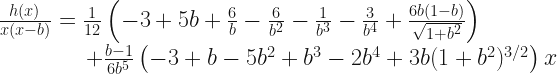
In part 2, we discussed some analytic results that one could obtain from this very difficult problem. We showed or argued that there were two transformations that mapped an optimal path on one road to another optimal path on a different road. Then, we used perturbation theory to approximately solve the problem in the case where traffic on the road was light. We will want to compare the results from this part to the perturbative results, so I will quote them here. We expanded the function representing the path to second order in $\lambda$ .

$f(x) = \frac{x}{b} + \lambda g(x) + \lambda^2 h(x) +\mathcal{O}(\lambda^3)$

We then used the equation of motion (which can be found in part 2) to find $g(x)$ and $h(x)$ .

$g(x) = \frac{1}{2}\left(\frac{1}{b^3} - \frac{1}{b^2} + \frac{1}{b} - 1\right)x(x-b).$

$\frac{h(x)}{x(x-b)} = \frac{1}{12} \left( -3 + 5 b + \frac{6}{b} - \frac{6}{b^2} - \frac{1}{b^3} - \frac{3}{b^4} + \frac{6 b (1-b)}{\sqrt{1 + b^2}} \right)\\ \phantom{00000000}+ \frac{b - 1}{6 b^5}\left( -3 + b - 5 b^2 + b^3 - 2 b^4 + 3 b (1 + b^2)^{3/2}\right) x$

With this information, we can now discuss our final attempt at solving this problem, putting it onto a computer. We will go over the process of how to reformulate the problem so that a computer can actually handle it, and then we will compare these non-perturbative solutions to those we obtained with perturbation theory in the last part.

Discretization – Overview

Our problem is based in calculus: we want to minimize a functional ( $E[f]$ ) over a space of functions. This all sounds very continuous, but computers cannot handle anything continuous. That is because any continuum contains an infinite amount of information. Even just the number $\pi$ cannot be represented exactly on a computer because it has an infinite number of digits, without a pattern. Therefore, on a computer, we can only get approximate answers, as we did in perturbation theory. Unlike perturbation theory, however, we don’t have to be restricted to small parameter values.

Before we get into the how of discretization, we should discuss the what, that is, what is it that we want to discretize? In part 2, we saw the expected distance functional and the equation of motion. Depending on taste, we could use either one of these to solve the problem. In this post, we will be discretizing the functional. As someone who isn’t too comfortable with more sophisticated computational methods, this is the easier option. The goal is then to calculate the expected distance for some path and then try to deform the path so that we are always decreasing the expected distance.

We want to discretize a functional. How do we do it? The fundamental object in our model is the path. The path is continuous, which is bad for a computer, as we described above. Therefore, we will have to discretize the path in order for the computer to be able to calculate with it. We will see that once the path is discretized, everything else will be calculable on the computer.

Discretization in Action

We want to discretize the path. In other words, we want to chop up the path into a finite number of simple bits so that the computer will be able to handle each one. Let’s take each bit of the path to be a straight line. We will see that this will make computations easier than other possible options.

A sketch of a graph. Above each marked value on the x-axis, there is a red dot, placed at some height between 0 and 1. The dots extend out to an x value of b, with each dot being separated horizontally by a distance called delta x. The first dot is located at the origin, and the last dot is located at the point (b,1). Adjacent dots are connected by a straight red line, representing the path of the walker. — The path can be represented by a finite number of points, connected by straight lines.

We will say that there are $N+1$ points (including the end points), each separated horizontally by a distance $\Delta x=b/N$ . The straight lines connecting these points represent the path of the walker. By increasing $N$ , we increase the accuracy of our calculation (by making the path look smoother/more continuous).

Once we have discretized the path, the rest is easy! Everything else we need in order to calculate $E[f]$ is just taking integrals of fairly simple functions. The arclength is just the length of a bunch of straight lines (which doesn’t even require an integral), and the remaining integrals are just those of exponentials and exponentials times linear functions, which are both things that can just be written down. So, given a path, we can write a sum of elementary functions that will produce the expected distance of that path. Then what?

If we want to find the minimum expected distance, then we are going to want to deform the path in such a way that the expected distance decreases. There are different methods of doing this (I personally implemented two different ones), but we are going to focus on gradient descent. We can imagine the space of discretized paths as living in an $(N-1)$ -dimensional space, $\mathbb{R}^{N-1}$ (specifically the unit cube in that space, since we are only considering functions from $[0,b]\rightarrow[0,1]$ ), where each dimension corresponds to one of the points we use to construct our path. We can then calculate the (approximate) partial derivative of the expected distance function in each “direction” to obtain the gradient. To get the partial derivative in the $i^{\text{th}}$ direction, we just move the $t^{\text{th}}$ path point by a small amount, $\delta x$ , and recalculate the expected distance. The partial derivative is then approximately given by $(E'-E)/\delta x$ , where $E'$ is the recalculated value of the expected distance. Once we have the gradient, we know the direction in our $(N-1)$ -dimensional space that corresponds to going uphill. We want to go downhill, so we take a step in the opposite direction. We keep doing this until we think we are at the lowest expected distance value.

Because we can’t know for sure whether we are at the minimum, we just say that since the gradient disappears at the minimum, we should keep descending until the gradient becomes very small (where we have to decide what “very small” means). That way, when we stop, we should be near a minimum. There are some subtleties here about local vs. global minima, but we will ignore those in this post.

As you might expect, the code runs more quickly with smaller values of $N$ , so as a little optimization trick, I wrote the code such that it begins with $N=2$ (one free parameter), and then after it optimized at that path, I divided each line of the path in half, doubling $N$ , and beginning the next gradient descent from that position. This allows the code to get through the large-scale deformations of the path quickly, and work its way to finer and finer detail. The code stops once the $N=64$ path is considered optimized. All paths begin as straight lines from origin to destination, before the gradient descent begins.

Results

Let’s dive into the results of the computational scheme outlined above. We will do a brief survey of solutions, stepping through different values of $b$ and $\lambda$ . Then, we will briefly test the analytic claims from part 2: the mirror symmetry, self-similarity, and results from perturbation theory. This will allow us to also see how far perturbation theory can take us.

Animated gif of a street of length 0.5. There is a number in the bottom right corner displaying the traffic rate, cycling through (0.25, 0.5, 0.75, 1.0, 1.5, 2.0). As the traffic rate increases, the optimal path goes from approximately linear to sagging more and more downward. — Optimal solutions generated on a street of length 0.5, for varying traffic rates, displayed in the corner.

Animated gif of a street of length 1.5. There is a number in the bottom right corner displaying the traffic rate, cycling through (0.25, 0.5, 0.75, 1.0, 1.5, 2.0). As the traffic rate increases, the optimal path goes from approximately linear to arching higher in the center. — Optimal solutions generated on a street of length 1.5, for varying $latex traffic rates, displayed in the corner.

Animated gif of a street of length 2. There is a number in the bottom right corner displaying the traffic rate, cycling through (0.25, 0.5, 0.75, 1.0, 1.5, 2.0). As the traffic rate increases, the optimal path goes from approximately linear to arching higher and higher. At a traffic rate of 1.0 and up, the optimal path has arched so high that it reaches the other side of the street before reaching the destination, then it continues horizontally to finish the path. This horizontal piece gets larger as the traffic rate continues to climb. — Optimal solutions generated on a street of length 2, for varying traffic rates, displayed in the corner.

The above animations are displaying the optimal solutions for three different road lengths, 0.5, 1.5, and 2.0, and each frame of the animation represents a different traffic rate. There are some qualitative features that we should make note of, which seem to hold in general. For roads of length less than 1, the optimal path is concave up, whereas for roads of length greater than 1, the optimal path is concave down. This fits with the mirror symmetry property we looked at in part 2. The other major qualitative feature appears when $b$ and $\lambda$ get to be large enough. The optimal path reaches the other side of the road before reaching the destination. This is an interesting feature that we would not get out of perturbation theory, since it fails at these large values of $\lambda$ .

Mirror Symmetry

In part 2, we made the claim, with a rough idea of a proof, that there is a transformation that maps solutions on a $1\times b$ road with traffic rate $\lambda$ to solutions on a $1\times1/b$ road with traffic rate $b\lambda$ . The transformation was simple, just take the inverse of the path function and re-scale distances appropriately so that the path starts and ends at the right points. I simulated this for the $b=2,\,\lambda=0.5$ case, with the dual path having $b=0.5,\,\lambda=1$ . Taking the dual path, flipping it across the line $y=x$ , and re-scaling, we see beautiful agreement between the two solutions.

There is one difficulty in producing these sorts of plots, which exposes a downside of using this particular algorithm. When using values of $\lambda$ which are particularly large on a road with $b>1$ , the slope of the path becomes very small near the destination. When considering the dual path, this corresponds to a very large slope. However, the slope is limited by the range of values that the discrete path points may take. For a road with $b=1/2$ , like in the dual path above, slopes are limited to $b/N = 1/128$ , and that is only if a point is at 0, with the next point at 1. This constraint leads to issues at these larger values of $\lambda$ , in the region where the slope must start growing to be very large.

Self-similarity

The self-similarity property was also laid out in part 2, though it was only an argument, without even a suggestion of a proof outline. We will test that claim now. The proposal was that, starting with the optimal path, one could remove some portion of the beginning of the path, then translate and re-scale everything so that we had a new, valid set-up. This would produce another optimal path on a different road with a different traffic rate.

In more detail, say we have an optimal path, $f(x)$ on a $1\times b&s=1$ road with traffic rate $\lambda$ . If we cut off the path between the origin and $x=s$ , then we would translate the path back so that it started at the origin, and re-scale distances and times so that the new path, $(f\left([1-f(s)]x+s\right)-f(s))/(1-f(s))$ , is optimal on a $1\times(b-s)/(1-f(s))$ road with traffic rate $(1-f(s))\lambda$ .

To test this, I used the optimal path on a $1\times 2$ road with traffic rate $\lambda=2$ , and then cut off the path up to $x=0.5$ , with $f(0.5)=0.4608$ . Using the transformation above, that gave a new road with dimensions $1\times2.7819$ and traffic rate $\lambda=1.0784$ . Here is a plot of the optimal paths of each of these roads, superimposed and restricted to the region where they overlap:

Plot showing excellent agreement between two paths related by the self-similarity property. — The optimal path on a street of length 2 and traffic rate 2 in blue, and on a street of length 2.7819 and traffic rate 1.0784 in orange. The latter has been transformed to show the self-similarity property by being properly scaled and translated so that it overlaps with the former path. Only the overlapping region is shown. The points don’t line up because the blue path has been cut off, while the orange path has not.

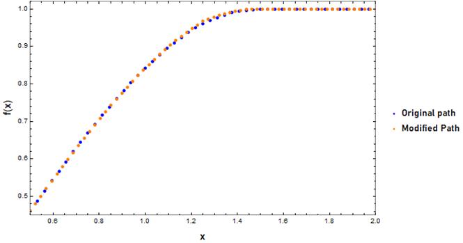
I was very confident when laying out the mirror symmetry property in part 2 because I had done the proof myself. When it came to the self-similarity property, I was less sure, though I felt the argument was very persuasive. When I published part 2, I hadn’t yet checked whether the self-similarity property held using my code. This was a bit nerve-wrecking, but I am pleased that it turned out alright.

Comparing to Perturbation Theory

Let’s compare the results from the code to those that we obtained using perturbation theory in part 2. Let’s quickly recall the perturbative results. The path is expanded in powers of $\lambda$ ,

$f(x) = \frac{x}{b} + \frac{\lambda}{2}\left(\frac{1}{b^3}-\frac{1}{b^2}+\frac{1}{b}-1\right)x(x-b)+\lambda^2 h(x)+\mathcal{O}\left(\lambda^3\right)$ .

We are going to ignore the $\mathcal{O}(\lambda^2)$ term except to say that it actually makes the approximation worse. This may be remedied at higher order, or may be indicative of a divergent series. But we don’t need to get into that. Below, we will show a couple different possible roads with different values of $\lambda$ , comparing the results from the algorithm to perturbation theory.

Animated gif of a plot of the optimal path as orange dots, on a street of length 0.75, cycling through traffic rates 0.5, 0.75, and 1.0. There is a blue curve representing the approximate solution from perturbation theory. As the traffic rate increases, the approximation gets worse, but not by much. — In orange, the optimal path on a street of length 0.75, for varying traffic rates displayed in the corner. In blue, the approximate solution from first order perturbation theory.

Animated gif of a plot of the optimal path as orange dots, on a street of length 1.5, cycling through traffic rates 0.5, 0.75, and 1.0. There is a blue curve representing the approximate solution from perturbation theory. As the traffic rate increases, the approximation gets worse. At a traffic rate of 1, there is a very noticeable difference. — In orange, the optimal path on a street of length 1.5, for varying traffic rates displayed in the corner. In blue, the approximate solution from first order perturbation theory.

These show how good the approximation is as $\lambda$ gets larger. At larger values of $b$ and $\lambda$ (both equal to 2, say), the first order approximation hits an issue, where it takes values above 1. This is nonsensical in the context of our problem, so there are specific points where we know that first-order perturbation theory ceases to work. However, as expected, the first order approximation works just fine for smaller values of $\lambda$ . It also appears as though the scale $\lambda_{max}$ at which this approximation breaks down decreases as the length of the road gets further from 1.

Conclusion

That concludes this series. We looked at a model of a pedestrian crossing a road, with limited prior knowledge of when cars would appear. Then we tried to optimize a path across the road which would take the least amount of time on average. We used symmetry arguments to obtain non-perturbative information about optimal paths, and we used perturbation theory to obtain approximately optimal paths, which were valid for small enough traffic rates. In this post, we placed the optimization problem on a computer by discretizing the path and implementing a gradient descent algorithm to find the smallest expected distance. Then, we used this code to verify the symmetries of the problem and test the robustness of the first order perturbative solution.

Are there any applications of this to the real world? To be honest, I don’t really care about that, I just wanted to answer this question that I’ve been thinking about for a number of years. However, I could see some weird future, where Amazon warehouses are staffed by robots wheeling around to relocate items. These results could be used to make an algorithm that would improve efficiency when it comes to robots not crashing into each other, but quicker. If Amazon wanted to, I hope they’d at least give me some money for it.

Quick Recap

Discretization – Overview

Discretization in Action

Results

Mirror Symmetry

Self-similarity

Comparing to Perturbation Theory

Conclusion

Share this:

Like this:

Related

Leave a Reply Cancel reply