Crossing the Street – Pt. 1

In this level 2 post, we start the process of a 3-part mathematical modelling series, which will culminate in the answer to one of the most important questions of all time: How should I cross the street?

Introduction

For quite some time now, I have been thinking of a fun problem, and I thought it would be interesting to do a series of posts about it detailing the basics of mathematical modelling. This first post in the series is about the set-up, where we take a real life situation and transform it into mathematics. This process is an essential skill to those pursuing physics and applied mathematics. The best way to learn is by example, so I figured this would be a great way of sharing this fun problem.

The particular problem is one that I have been thinking about off and on for somewhere around 15 years. That’s more than half of my life! It first came to me when I was in elementary school, walking home, and trying to get there quickly. I was on the right street, but the opposite side of the road to my destination. It was a residential street, so I knew cars wouldn’t come very often. I started crossing the street in a sort of diagonal manner, constantly looking down the street in each direction for cars. Of course, if a car came, I would have to make a hard left and get out of the road, and this got me thinking about whether I was taking the best path across the street. The shortest path was the straight line, sure, but the fact that I would have to vacate the road when a car came makes the whole situation a bit different. At the time, I would have had no idea about how to actually find the answer to this question, and it wouldn’t even be until graduate school until I could confidently formulate it. But as a child, my intuition was that the best course would be one that sort of arcs around the straight-line path, at first more directly crossing the street, then to curve down the road more parallel to the curb. I though of it kind of like landing a plane on the opposite curb.

The problem sprung to mind every now and again, whenever I was doing a lot of walking around town, and not too long ago, it came back. I realized that this was a problem that I could model, and potentially solve once and for all. For the past couple of years, I have been noodling around with this problem whenever I didn’t feel like doing anything else (graduate students don’t really have all that much free time). This is the culmination of that work.

The Basic Components

We should start by taking the critical components of this real-life situation and abstracting them into something we can represent with mathematics. Let’s take things one component at a time.

The Street

This is the easiest component to deal with, so it goes first. We only care about the portion of the street between the walker and their destination, and we won’t consider any winding roads. For a first model, we want to keep things relatively simple. The relevant section of the road is just a rectangle, with a width $A$ and a length $B$ . The walker starts on one corner of this rectangle, and the destination is at the opposite corner. To be concrete, let’s set up a coordinate system where the walker starts at the origin, and the destination is at the point $(B,A)$ .

Diagram of a road running left to right, with a set of coordinate axes running along the left and bottom sides of the road. There is a red dot at the lower left corner, indicating the starting position of the walker, and a red 'x' in the upper right corner, representing the destination. There are markings on the axes at the horizontal and vertical positions of the destination. The vertical position is labeled with a capital 'A', and the horizontal position is labeled capital 'B'.

The Walker

What do we need from the walker? Well, they have to have a position (we set them at the origin at the beginning), and they are going to walk along a path that we will pay specific attention to separately. Let’s model the walker as a point, which has a definite position at any given point in time. The fact that a person is an extended object isn’t relevant to the particular problem, so we don’t have to think of them as anything more than a point. In many physics models (especially in intro physics courses), this is often implied, but I want to make things as explicit as possible.

The only other thing we need from the walker is for them to… well, walk. The speed at which the walker travels is going to be important because if the walker is very slow, there is a bigger chance that they will see a car before they reach their destination. To make things as simple as possible, we will assume that the walker walks at a constant speed, which we will call $v$ .

The Car

Now we are getting into some real modelling choices. The car is referred to as the car because we don’t care if there are any more after. Once there is one car, the walker is going to get out of the way and that’s that. They are already on the correct side of the street, so there’s no use getting back into the road.

We don’t know when the car will arrive, since cars don’t follow rigorous schedules, they get held up in traffic, sometimes the driver is running a little late or early, etc. The next best thing would be to know about how often cars show up on the road on average. This sounds like we are going to need some probability theory. In particular, we are going to model the car’s arrival as a Poisson process. A Poisson process is one that happens at random, but with an average rate which we can call $\Lambda$ . The usual story is that if you arrive at a bus stop, and the bus is not there, the probability density of the next bus arriving in the next $t$ minutes is given by the Poisson distribution,

$\rho(t) = \Lambda e^{-\Lambda t}$ ,

where $\Lambda$ is the average rate at which buses arrive at the stop. In other words, the probability of the next bus arriving in a tiny time interval between $t$ and $t+dt$ is

$P([t,t+dt])=\rho(t)\,dt=\Lambda e^{-\Lambda t}\,dt$ .

Then, for a larger interval, we just integrate. If it works for buses, this seems to be a reasonable model for our car. Say that the moment the walker begins on their path is the time $t=0$ . We should also name the time at which the next car arrives, so let’s call that $t_*$ .

The Path

The path is a little tricky. Really, there are two paths: the intended path and the actual path. The intended path is the path that the walker would take if a car never showed up. The actual path is the path that the walker actually takes, which can be diverted should a car come. Let’s focus first on the intended path.

The intended path can be abstracted in several ways, but let’s start general, and see if we can do anything to make our model (and lives) simpler. The path can be written in a parametric form, $(x(t), y(t))$ . This parametric form allows us to do all sorts of fun things with our intended path, we could have the walker do loops and meander all over the place, doubling back on themself and so on. But our final goal is to find an optimal path. Certain behaviors are not going to give us an optimal path. For example, we can easily argue that walking away from the destination will result in a less-than-optimal path because we can always cut off the part of the path that doubled back to create a better path. I am not going to provide some rigorous proof of this idea, but below, you can see a sketch of what I mean.

A two-panel sketch. In each panel there is a different path. In the left panel, the path begins going to the right, then swerves back to the left, and finally swerves back to the right again. In the right panel. the path begins going to the right, then goes straight upwards, and finally turning rightward again. There is a dotted line representing the part of the path in the left panel that is "cut off" by this procedure. — Building a better path from one that turns back on itself in the horizontal direction

A two-panel sketch. In each panel there is a different path. In the left panel, the path begins going upwards, then swerves back in a downward direction, and finally swerves back to going upward again. In the right panel. the path begins going upwards, then goes straight to the right, and finally turns upward again. There is a dotted line representing the part of the path in the left panel that is "cut off" by this procedure. — Building a better path from one that turns back on itself in the vertical direction

When we cut off these unnecessary parts of the intended path, we can see that a parameterization is a little too general. Cutting off the horizontal jog in the first diagram ensures that the path can be represented as a function of $x$ . Moreover, the fact that we can also cut off the vertical jog means that this function is never decreasing. Let’s give this function a name: $f(x)$ . You will notice that this is not explicitly time-dependent, like the parameterization was. Just think of this as implicitly depending on time for now. We will address this later. The only other thing to mention about the intended path function is that it must start at the origin and end at the walker’s destination, which in terms of the math is, $f(0)=0$ and $f(B)=A$ .

Now we can discuss the actual path. What happens when a car comes? Before, we said that the walker diverts themself off the intended path and onto the other side of the street, but to treat this mathematically, we need to know exactly how this diversion happens. Simplicity is the main driver of our model, so let’s say that the diversion is to immediately finish crossing the street, and then finish walking down the road to the destination, as shown in the figure below.

Sketch of a rectangular section of road with a set of coordinate axes running along the left and bottom sides of the road. There is a red dot in the lower left corner, indicating the walker's starting position, and there is a red 'X' in the upper right corner indicating the destination. A red path is depicted, starting at the walker's starting point and traveling in a winding manner towards the destination. Near the middle of the road, a car is said to have appeared, so the path abruptly turns to go in the vertical direction until it reaches the top side of the road, and proceeds to the right to the destination. A red dotted line indicates where the path could continue if the abrupt turn had not occurred. — The intended path of the walker is interrupted by oncoming traffic, resulting in the actual path. The rest of the intended path is drawn as a dashed line

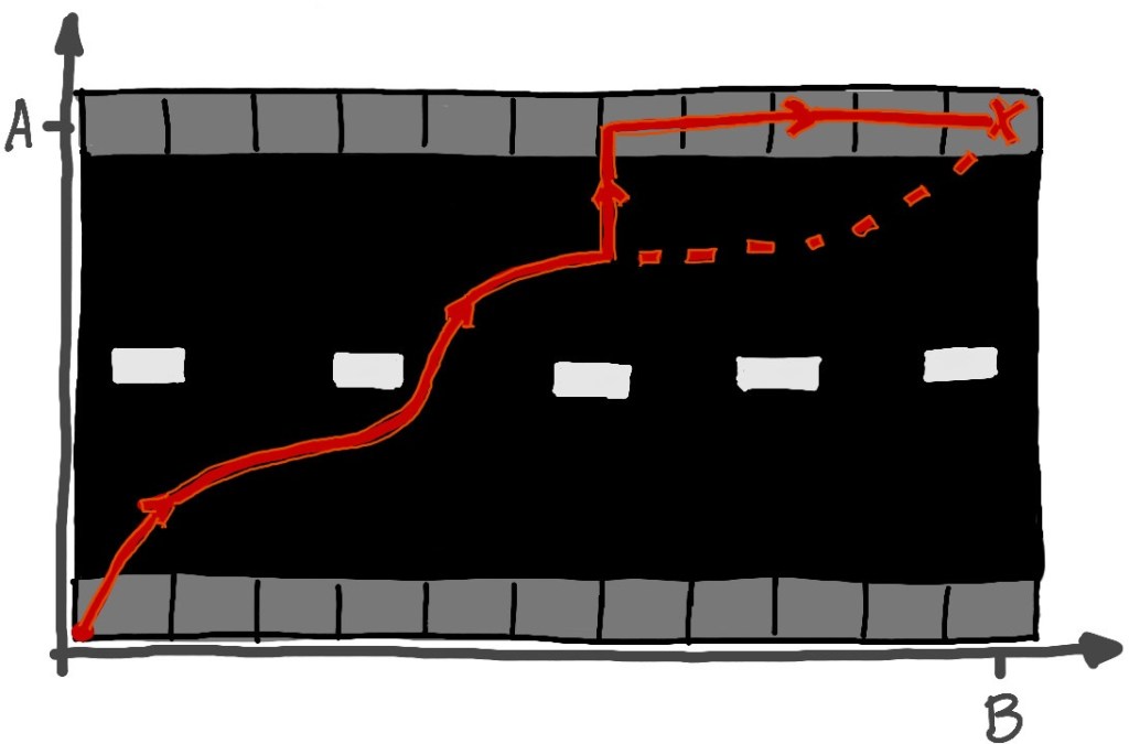
This particular model of the actual path makes calculating distances very easy. The additional distance traveled once the car appears is just 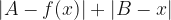$|A-f(x)|+|B-x|$ .

Nondimensionalization

So far, we have a model that consists of several parameters: the lengths of each side of the street, the speed of the walker, and the rate at which cars appear on the road. Four may not seem like many parameters, but in any model, it is best to reduce the number of parameters to as small a set as is possible. One particularly nice way of doing so is called nondimensionalization, and as the name implies, it is about getting rid of the unnecessary “dimensions” of the model. By dimensions, I mean units (like seconds, meters, kilograms, etc.).

We have two relevant units in this problem: length and time. By choosing our particular units of measurement, we can actually cut down on parameters in the model. For example, in high energy physics, we typically choose our units so that the speed of light is equal to 1. Think of the time units as seconds and the length units as light-seconds (the distance light travels in a second). Clearly, in these units, the speed of light is 1 light-second per second. But when we say that the speed of light is 1, we actually mean something even more. The number 1 is unitless, it doesn’t have units of light-seconds per second. This means that in this system, all speeds are just numbers and the units of length and time are the same (like saying a distance of 2 seconds is the distance light travels in 2 seconds). When we are done making predictions, we can reintroduce standard units back into the picture by taking any prediction of lengths (in our weird units where length is in seconds) and multiplying by the speed of light in meters per second, making it a distance in meters. Let’s apply this to our model.

The exact dimensions of the street are not too important to us. We really just care about the overall shape of the rectangle, so we can choose one of the sides to be our unit of distance (making it have length 1). Let’s say that the width of the road is 1, that is $A=1$ . This will affect the other length in the problem. In these new units, the length of the road is now $b=B/A$ . When we want to use our results on a real road, we just need to reintroduce the length units by multiplying by $A$ , and that will return us to the original $B$ .

Now let’s get rid of the time units. There are two ways of doing this, by setting $\Lambda=1$ or by setting $v=1$ . Both of these parameters encode information about how likely it is that the walker will see a car before reaching their destination. A quicker walking speed would mean that the walker is less likely to see a car, just as a lower rate of traffic would. I would argue that it is more natural to set the walking speed to 1 because that is fixed by the person, whereas the rate at which cars come is a parameter that I would like to dial. We want to see what happens when the road never has cars on it, and when it has many cars on it, which is a large range of $\Lambda$ , but there is an upper bound on walking speeds (no one is going to be walking at a mile a minute, for example), so $v$ has a comparatively small range of typical values. With this choice, our unit of time is the amount of time it would take the walker to directly cross the street. We can call our nondimensionalized rate $\lambda = A\Lambda/v$ . This rate is how many cars on average appear on the road in the time it takes the walker to cross the street directly.

Our Model

Now that we have all the pieces, we can put everything together into a working model. To do so, we must answer one big question: what does it mean to be the “best path”? There may be several different good answers to this question, but to me, two possibilities stand out. We should either decide that the best path is the one that is the shortest distance (on average) or that the best path should be the path with the shortest travel time (again, on average). Luckily for us, we don’t have to choose between these two options because the walker has a speed of 1, so these turn out to be the same question in this model. To be concrete, we will always think in terms of distances. This will make the problem technically simpler, but I would also encourage the curious to reformulate everything in terms of times to see how this affects the governing equations of the model.

How would we calculate the average distance traveled by the walker? Let’s start by calculating the distance traveled on the actual path, when a car comes. Say that at the moment a car comes, the walker is at the $x$ -coordinate $x_*$ . Then, the distance traveled by the walker will be the arclength of the intended path up to that point, plus the extra distance we add to make the actual path. For now, we will just call the arclength from the origin to $x_*$ , $A(x_*)$ .

$D(x_*) = A(x_*) + |1-f(x_*)| + |b-x_*|$

Now, in order to calculate the average value, we need the probability associated to each possible distance. We have the probability distribution for a car to arrive at a particular time, but we would like to instead have the probability distribution for a car to arrive when the walker is located at a particular location. The time and $x$ position are related by

$vt = A(x)$ ,

where I have included the $v$ to make things more intuitive, but of course, the speed is still 1. This is all we need to do the conversion, so long as we are careful. We shouldn’t just shove this into the probability distribution, we need to transform the probabilities themselves. The probability of a car arriving between time $t$ and $t+dt$ is given by

$\rho(t)\,dt$ .

We need to also transform that differential $dt$ . In more formal language, we are dealing with not just a probability distribution, but a probability measure. Now, we can rewrite the probability measure in terms of $x$ .

$\rho(t)\,dt = \rho(A(x))\,\frac{d}{dx}A(x)\,dx = \lambda A'(x)\text{exp}(-\lambda A(x))\,dx$

Now, the expected distance traveled by the walker is given by a sum of the possible distances traveled, multiplied by the probability associated with each distance.

$E[f] = \lambda\displaystyle\int_0^b A'(x)e^{-\lambda A(x)}D(x)\,dx + A(b)e^{-\lambda A(b)}$

I snuck in that last term there without talking about it, so I better fess up. The last term takes into account the possibility that the car does not come before the walker reaches their destination. But you will notice that it is in the form of a distance (the full arclength of the intended path), multiplied by the probability that the car does not come before the walker finishes their journey. This term can be calculated explicitly as an integral (easier when expressing everything in terms of time), so if you are curious how it got there, just do the integral.

Our model is now complete! Our goal from now on will be to find the path that minimizes the expected distance. To see the explicit dependence of the expected distance on the path, I will write everything out in full.

$E[f] = \lambda\displaystyle\int_0^b\sqrt{1+(f'(x))^2}\,e^{-\lambda\int_0^x\sqrt{1+(f'(y))^2}\,dy}\left[\int_0^x\sqrt{1+(f'(z))^2}\,dz + |1-f(x)| + |b-x|\right]\,dx \\ \phantom{\left[\int_0^x\sqrt{1+(f'(z))^2}\,dz + |1-f(x)| + |b-x|\right]}+ e^{-\lambda\int_0^b\sqrt{1+(f'(x))^2}\,dy}\displaystyle\int_0^b\sqrt{1+(f'(x))^2}\,dx$

This is a very non-linear problem. We will try some methods at solving this problem in parts 2 and 3 of this series, but for now, let’s gain some intuition for how our model works.

Limiting Behavior

Looking at the limiting behavior of a model is a great way to understand some fundamental features of a model and can also act as checks on calculations to ensure there aren’t mistakes. By “limiting behavior”, I simply mean what we expect to be true of the model in extreme circumstances. In this case, we should look at extreme values of the parameters of our model and gain some intuition about what the best path should look like in these cases.

Let’s start with $b$ . In the case where $b$ is very small (compared to 1), any non-decreasing function with endpoints at $(0,0)$ and $(b,1)$ will look very much like a straight line. The difference between, for example, the straight-line solution and the longest reasonable solution (where you just cross the street directly) is negligible for small $b$ :

$(1+b)-\sqrt{1+b^2} = (1+b)-(1+\mathcal{O}(b^2)) = b+\mathcal{O}(b^2)$ .

In this case, the expected distance is virtually identical across all paths. If you could imagine the expected distance graphed over function space, it would become very flat around the optimal path in this limit.

A similar thing happens in the limit of large $b$ . Let’s again look at the difference between the straight-line solution and the longest reasonable solution in this case:

$(1+b) - \sqrt{1+b^2} = (1+b) - b\sqrt{1+\frac{1}{b^2}} = 1+\mathcal{O}\left(\frac{1}{b}\right) \ll b$ .

Here, the expected distance is also nearly identical across all paths. This is telling us that if there is any interesting behavior, it will be when $b$ takes on intermediate values (when $b$ is of order 1, in theoretical physics lingo).

Now, let’s look at $\lambda$ . For very large $\lambda$ , the car is very likely to appear as the walker takes their first step. Therefore, the intended path is mostly inconsequential, as the walker is almost never going to follow it past that first step. This situation mirrors what happens for extreme values of $b$ , where the expected distance graph looks very flat in function space.

Finally, the small $\lambda$ limit has some different expected behavior. In fact, the limit is not entirely necessary because setting $\lambda=0$ makes sense. It just means that there are no cars. With no possibility of diverting the walker, the shortest path becomes the geometrically shortest path, i.e. the straight line. We can see from the expected distance formula that setting $\lambda=0$ reduces the problem to the problem of finding the path that minimizes the arclength. This is an important result that we will use when we tackle this problem analytically. Like $b$ , the simple limiting behavior in $\lambda$ implies that any interesting behavior in the problem will show up when $\lambda$ is of order 1, that is, when the walker has a decent chance of seeing a car during their journey. That concludes the limiting cases, and this first post about modeling this street-crossing problem.

I am expecting to post part 2 in one week, and part 3 the following week. In part 2, we will be looking at ways of tackling this highly non-linear problem analytically. In part 3, we will take a swing at discretizing the problem, so that it may be solved on a computer. I hope that spacing things out in this way will allow those of you who are curious to have some time with this problem before I post my solution(s). You can leave a comment below if you find anything interesting about this problem. See you next week!

2 thoughts on “Crossing the Street – Pt. 1”

Pingback: Crossing the Street – Pt. 2 – Singular Points
Pingback: Crossing the Street – Pt. 3 – Singular Points