Crossing the Street – Pt. 2

In the 2nd part of this level 2 mathematical modelling series, we take a look at what sorts of analytical tools we have to address the problem of how best to cross the street.

Quick Recap

In part 1 of this series, we built a mathematical model of a person crossing the street. We modeled the road as a $1\times b$ rectangle, with one corner at the origin and the opposite corner at the point $(b,1)$ . Cars appear on the road at random, but with average rate $\lambda$ . The walker starts at the origin and walks along a path, represented as a function $f(x)$ that is non-decreasing. We were trying to find the intended path of the walker that minimized the distance traveled. In the end, we had the expected distance traveled in terms of the path:

$E[f] = \lambda\displaystyle\int_0^b\sqrt{1+(f'(x))^2}\,e^{-\lambda\int_0^x\sqrt{1+(f'(y))^2}\,dy}\left[\int_0^x\sqrt{1+(f'(z))^2}\,dz + |1-f(x)| + |b-x|\right]\,dx \\ \phantom{\left[\int_0^x\sqrt{1+(f'(z))^2}\,dz + |1-f(x)| + |b-x|\right]}+ e^{-\lambda\int_0^b\sqrt{1+(f'(x))^2}\,dy}\displaystyle\int_0^b\sqrt{1+(f'(x))^2}\,dx.$

In this second part, we are going to use some analytic techniques to obtain some exact information, as well as some approximate solutions to the problem, using symmetry arguments and perturbation theory.

Equation of Motion

Although we have an expression for the expected distance, we haven’t established how to systematically decide what the best path is. How do you go from “we need to minimize this expression with respect to the path” to actually doing that. The answer is in a branch of mathematics called the calculus of variations (or variational calculus), and it is widely used in modelling and physics. The idea behind variational calculus is to use calculus to minimize a functional (like what we have) in a similar way that we would minimize a function in ordinary calculus: find the point where the derivative is 0.

As this is a series on modelling and not variational calculus, I will skip the details of the variation. Plus, it is a very messy calculation, and I don’t want to type all of it out. The end result of variational calculus is almost always an integro-differential equation, which is a lot like a differential equation, but it can also contain integrals. This is often called the Equation of Motion (EoM) in physics, and I will use that term here as well.

The Equation of Motion

In full, the EoM is:

$0=f''(x)\left[\,e^{-\lambda\int_0^b\sqrt{1+f'(z)^2}\,dz}\left(\lambda\displaystyle\int_0^b\frac{dy}{(1+f'(y)^2)^{3/2}}-1\right)-\lambda\displaystyle\int_0^x\,e^{-\lambda \int_0^y \sqrt{1+f'(z)^2}\,dz}\,dy\right] \\ +\lambda^2f''(x)\displaystyle\int_0^x\sqrt{1+f'(y)^2}\,e^{-\lambda\int_0^y\sqrt{1+f'(z)^2}\,dz}\left[\int_0^y\sqrt{1+f'(z)^2}\,dz +1-f(y)+b-y\right]dy\\ \phantom{000000000000000000}-\lambda f''(x)\,e^{-\lambda\int_0^x\sqrt{1+f'(z)^2}\,dz}\left[\int_0^x\sqrt{1+f'(z)^2}\,dz+1-f(x)+b-x\right]\\ \phantom{0000000000000000000000000000000000}+\lambda\,e^{-\lambda\int_0^x\sqrt{1+f(z)^2}\,dz}\left[f'(x)^3-f'(x)^2+f'(x)-1\right]$

This is a little simpler if we rewrite everything in terms of the arc length function, $A(x)$ and the distance function, $D(x)$ which we defined in part 1 to be:

$A(x) = \displaystyle\int_0^x\sqrt{1+f'(z)^2}\,dz,\\D(x)=A(x)+1-f(x)+b-x$

In terms of these functions, the Equation of Motion looks like

$0=f''(x)\left[\,e^{-\lambda A(b)}\left(\lambda\displaystyle\int_0^b\frac{dy}{(1+f'(y)^2)^{3/2}}-1\right)-\lambda\displaystyle\int_0^x\,e^{-\lambda A(y)}\,dy\right] \\ \phantom{00000000000000}+\lambda^2f''(x)\displaystyle\int_0^x A'(y)\,e^{-\lambda A(y)}D(y)dy-\lambda f''(x)\,e^{-\lambda A(x)}D(x)\\ \phantom{000000000000000000000000000000}+\lambda\,e^{-\lambda A(x)}\left[f'(x)^3-f'(x)^2+f'(x)-1\right]$

This is a very complicated, non-linear integro-differential equation. Normally, when we encounter such beasts, we put our head in our hands and cry. Then we try to poke and prod at it until we can get something useful out of it. Finally, we just stick it on a computer and let it do the dirty work. We’ll leave the computer until part 3. For now, assuming that we are done crying, let’s poke and prod.

Symmetry

If we look at the problem closely, there are certain general statements that we can derive out of the structure of the problem itself. These are the symmetries of the problem. I am using the word ‘symmetry’ a bit loosely here, but in this section, we will look at certain transformations that map solutions to other solutions.

Mirror Symmetry

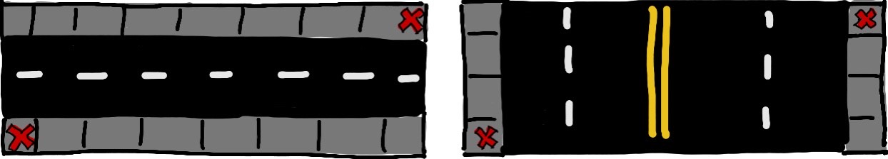
Up to this point, I have been drawing the road in such a way that traffic flows right-to-left and vice versa. However, nothing in the model specifies a particular direction of traffic flow. Since the road is just a rectangle in our model, traffic could be flowing upwards and downwards.

Sketch showing two roads, each drawn on rectangles of the same shape and size. On the left, the road is oriented such that traffic flows horizontally across the rectangle, and on the right, traffic flows vertically. — In each of these two diagrams, we have a section of road which has the same dimensions, but traffic flows in different directions.

The two roads above are treated exactly in the same way in our model because they have the same dimensions. But we could standardize the process, for example by requiring all the roads to have traffic that flows horizontally. This would require us to mess with the road on the right of the diagram so that it follows this new standardization. Although it is possible to do this in one step, I think a two step process is a little more intuitive. Let’s start by rotating the rectangle clockwise by one quarter turn, then flipping it across a vertical line.

Sketch showing the process of rotating and flipping the road so that it matches our new standard that traffic should flow horizontally.

Throughout this process, we want to make sure that the starting position of the walker remains at the origin, since that is specified in our model. That means that when we rotate the road a quarter turn counterclockwise, we want to rotate it about the origin. Then, when flipping the road, we want to flip it across the vertical axis, at $x=0$ . With these specifics, both transformations will leave the origin in place. Since we haven’t stretched or deformed the road in any way, the optimal path is still the best one, though it has also been transformed. The rotation and flip send the function $f(x)$ to its inverse. One way of seeing how that works is by noticing how the coordinate axes behave under these transformations. The rotation sends the $x$ -axis to where the $y$ -axis was, and the flip does nothing further. Meanwhile, the rotation sends the $y$ -axis the negative $x$ -axis, and the flip then sends it to the positive $x$ -axis. So the axes have swapped. All functions $y(x)$ now look instead like $x(y)$ , i.e. the inverse. This is why I have called this ‘mirror symmetry’. The quicker way of doing this transformation is just flipping across the line $y=x$ , which is usually how inverse functions are taught.

We aren’t quite done however. The destination is now at $(1,b)$ , whereas we specified in part 1 that everything should be scaled such that the destination is located at $(b,1)$ . Therefore, we need to divide our distances (and times) by $b$ . We now have a new solution on a road of different dimensions than before! The solution on one road gave us the solution on another road. In other words, if the intended path $f(x)$ is optimal on a $1\times b$ road with traffic rate $\lambda$ , then the intended path $f^{-1}(bx)/b$ is optimal on a $1\times 1/b$ road with traffic rate $b\lambda$ .

One way to make this rigorous is to take the expected distance functional and perform this transformation on it. What you will find is that the expected distance gets scaled by a factor of $1/b$ under this transformation. So not only is this useful for relating optimal paths to each other, but any path under this transformation will yield an expected distance will yield the original expected distance, divided by $b$ . This is exactly what we would expect! We get the same distance back because it is essentially the same problem, but it is scaled down by a factor of $b$ because we scaled all lengths down by a factor of $b$ . This also enforces the notion that the optimal path is mapped to another optimal path, because the minimum of a function stays the minimum even if you scale it down.

This is what I would call a duality, not a symmetry. This transformation relates a path on one road to a related path on a different road. However, this can be a symmetry if $b=1$ . Then, all the scaling is using a factor of 1, which of course does nothing. So on the square road, the mirror transformation maps a path to another path with the same expected distance. This is very suggestive. Although we haven’t shown that there is only one optimal path, and we won’t show that, and I don’t have a proof of that, we might hope that this is the case. The reason for this is that if there is only one solution, and there is a transformation that relates different paths with the same expected distance, then we have solved the problem on the square. To be explicit, a unique solution would be the path that is transformed to itself under the mirror transformation, which is the straight-line path. Indeed, if you input a straight line path, $f(x)=x/b$ into the EoM, you obtain:

$\lambda(b^{3}-b^{2}+b^{1}-1)\,e^{-\lambda\sqrt{1+b^{-2}}\,x} = 0$

Clearly, $b=1$ solves this equation. Therefore, the straight-line path is optimal on a square road, regardless of the traffic rate. This is quite a nice find! You might even notice that we have a cubic polynomial above, so there are two more solutions. However, these are both imaginary solutions, $b=\pm i$ , so we have just the one exact solution.

Because we can map optimal paths on rectangles with $b>1$ to optimal paths on rectangles with $0<b<1$ , we only have to solve the problem on one of these intervals.

Self-similarity

What is the probability of the car arriving in the next minute, if you have already waited 4 minutes without a car coming? You may be surprised to learn that it’s the same probability that the car would arrive in the first minute of you waiting. That is because when you have been waiting for 4 minutes without a car showing up, you have the extra knowledge that the car didn’t show up in those first 4 minutes. We cut off the first 4 minutes of the probability distribution and re-scale everything so that the total probability is 1. Because the probability distribution we have is exponential, this process returns the same thing that we started with. An animated version of this is included below.

Animation showing how a Poisson process has no memory.

The Poisson process that we chose to model the car is said to have no memory in the above sense. The probability distribution does not remember that you have been waiting 4 minutes already, it still says that the probability of a car arriving one minute from now is the same as the probability of a car arriving one minute from when you started.

This is a really interesting property of Poisson processes, and it leads us to our next “symmetry”. Let’s have the walker take a step along the intended path. Say that no car showed up during that moment. Because the Poisson process has no memory, the problem appears as though the walker never took that first step, and instead just started at their current location. Their goal is to now find the optimal path from where they are. After they take their next step, we could repeat the same reasoning. This is telling us that the problem is self-similar.

If you have the optimal path, then after every step, you also have an optimal path from that location, and so on. Let’s figure out how to frame this as a transformation between optimal paths. Say that after a step, the walker is now at the point $(s,f(s))$ . The rest of the path is now optimal on this smaller $(1-f(s))\times(b-s)$ street. But we are going to have to re-scale all of our dimensions to account for this new street shape. All distances and times will be scaled down by a factor of $(1-f(s))$ . The full transformation will be:

$b\rightarrow \frac{b-s}{1-f(s)},\phantom{000}\lambda\rightarrow(1-f(s))\lambda,\\ f(x)\rightarrow\frac{f([1-f(s)]x+s)-f(s)}{1-f(s)}.$

If you are unsure about the transformation of 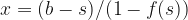$f(x)$ , note that this transformation gives the correct boundary conditions at $x=0$ and $x=(b-s)/(1-f(s))$ . There are no other transformations of this kind (translation+scaling) that produce the correct boundary conditions.

This is another useful transformation between optimal solutions on rectangles of different sizes, with different traffic rates. If we can solve the problem exactly for some values of $b$ and $\lambda$ , then we will have solved it for a whole continuum of other parameter values. I will be honest here and say that I haven’t rigorously proven this to be true, but I think this argument is persuasive.

For the physicists out there, this process reminds me of Renormalization Group flow, in that the parameters (couplings) run as you change the scale of the rectangle. It even flows to a fixed point, where $\lambda\rightarrow0$ and $b\rightarrow 1/f'(b)$ . There may be a way of starting at the fixed point and flowing away to give an exact solution to the problem, but I haven’t seen how this is possible. It would be analogous to RG flow away from the conformal fixed point of a quantum field theory. If anyone can write down an “RG equation” for this system, I would be very interested.

Perturbation Theory

Overview

Perturbation theory is an incredibly useful tool in the study of non-linear problems. The main idea is to take a parameter of the theory as a small number. The advantage of this is that solutions to the problem may be represented as a Taylor series in the small parameter, which is then computed order-by-order. We will see that this technique takes our very difficult non-linear problem and transforms it into an infinite number of easy problems, with each further easy problem becoming less and less important. Solving out to some finite order in the small parameter, we obtain an approximate solution to the problem.

In slightly more concrete terms, one should choose or insert the parameter such that the problem is exactly solvable when that parameter is set to 0. This gives us our order 0 solution, which will be used when we compute the order 1 solution, and so on until we give up.

Perturbation Theory in Action

We will use some ideas from the previous part of the series to choose our parameter. In our limiting cases, we saw that the $\lambda=0$ solution is just a straight line. This makes $\lambda$ the natural perturbation parameter. If we set $\lambda=0$ in our EoM, we obtain a very simple equation, $f''(x)=0$ , which verifies our previous reasoning that this yields a straight line. Now, write $f(x)$ as this straight line plus a contribution that is of order $\lambda$ ,

$f(x) = \frac{x}{b} + \lambda g(x) + \mathcal{O}(\lambda^2).$

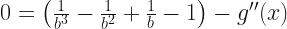
If we Taylor expand the EoM out to order $\lambda$ , we will obtain a differential equation for $g(x)$ .

$0 = \left(\frac{1}{b^3} - \frac{1}{b^2} + \frac{1}{b} - 1\right) - g''(x)$

The solution to the above equation will have 2 free parameters. We will set these with our boundary conditions on $g(x)$ . Since the full function must be 0 at $x=0$ and 1 at $x=b$ , and the order-0 solution already satisfies these criteria, then all the perturbations must vanish at the end points. That is, $g(0)=g(b)=0$ . The order- $\lambda$ solution is then

$g(x) = \frac{1}{2}\left(\frac{1}{b^3} - \frac{1}{b^2} + \frac{1}{b} - 1\right)x(x-b).$

I want to take a moment to examine this largest perturbative correction. Notice that the factor out in front is 0 at $b=1$ , which confirms what we know from the mirror symmetry. For $b$ between 0 and 1, this coefficient (and thus the second derivative of $g(x)$ ) is positive. For $b>1$ , this coefficient is negative. This gives us some important qualitative data about the path. On wide rectangles, the solution starts steep and levels off, whereas on narrow rectangles, the path starts shallow and gets steeper as the walker goes.

Animation of a rectangular section of road, which is growing and shrinking in length. There is a red curve going from the bottom left corner to the top right corner of the road. When the width of the road is smaller than the height, the curve is concave up, whereas when the width of the road is longer than the height, the curve is concave down. At the moment when the road is square, the curve is a straight line. — This animation shows the first order solution for different lengths of road. The dotted line shows the size of the square road, for reference.

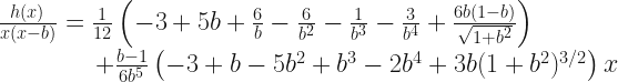
This suggests that even non-perturbatively, the solution could be concave up for $b<1$ and concave down for $b>1$ . We can’t know for sure until we have non-perturbative solutions, which will come in the next part, but this is a bit of intuition that we should keep around, as a conjecture for what solutions typically look like.

We can then plug $g(x)$ back into $f(x)$ and expand to order $\lambda^2$ .

$f(x) = \frac{x}{b} + \lambda g(x) + \lambda^2 h(x) + \mathcal{O}(\lambda^3)$

Expanding the EoM to order $\lambda^2$ yields a big, messy equation. However, it is just of the form

$0 = C(b) + D(b)x - h''(x),$

where $C(b)$ and $D(b)$ are just (very large and complicated) constants built out of $b$ . With the boundary conditions on $h(x)$ , this will just be a cubic polynomial.

$\frac{h(x)}{x(x-b)} = \frac{1}{12} \left( -3 + 5 b + \frac{6}{b} - \frac{6}{b^2} - \frac{1}{b^3} - \frac{3}{b^4} + \frac{6 b (1-b)}{\sqrt{1 + b^2}} \right)\\ \phantom{00000000}+ \frac{b - 1}{6 b^5}\left( -3 + b - 5 b^2 + b^3 - 2 b^4 + 3 b (1 + b^2)^{3/2}\right) x$

This, too, vanishes when $b=1$ , which is a fair indication that everything came out alright.

As is customary in physics, I am giving up after going to second order. In principle, you may continue this process as far as you like. The $n^{\text{th}}$ -order solution will yield a polynomial of degree $(n+1)$ . Assuming that the perturbation series for $f(x)$ converges, each extra term you compute will be more difficult with less reward for doing so. Perturbation theory is all about diminishing returns.

There is another parameter for which we know an exact solution, $b=1$ . In principle, one could do perturbation theory by sending $b\rightarrow1-\epsilon$ , and expanding in $\epsilon$ . I think there are some subtleties in this choice that I won’t go into, but if anyone tries this, let me know!

Conclusion

That is about all we will get to this time. It was a long one, and packed. We saw some symmetries of the street crossing problem, which allow us access to non-perturbative information. This came in the form of mirror symmetry, where the optimal path on one street was mapped to an optimal path on a different street. This lead us to one non-perturbative solution, the straight line solution, which is valid on the square road for any traffic rate. We also used the memorylessness of the Poisson process to argue that the problem is self-similar, which related a solution to an infinite family of related solutions, which all use the same path, in a sense.

Finally, we used perturbation theory to solve the problem for the case when the traffic rate is small. This gave us some useful qualitative information that hints at a non-perturbative fact about solutions for various lengths of road.

Next week, we will take a look at how to generate non-perturbative solutions to this problem by discretizing it and placing it on a computer. We can then check our results against the perturbative solutions to see how accurate they are. See you then!

One thought on “Crossing the Street – Pt. 2”

Pingback: Crossing the Street – Pt. 3 – Singular Points