Root-finding Fractals II

In this level 0 post, we revisit Newton’s method and the fractals it creates, but this time, we focus on generalizations of Newton’s method. This one’s for the people who love to look at fractals.

In my last post, we talked about Newton’s method and how it can be used to generate beautiful fractal images. I even wrote a JavaScript program [disclaimer, source code] so that you can create your own Newton fractal in your browser (now updated to include ideas from this post). The previous post set up the main ideas behind Newton’s method, so I wanted to make a follow-up that’s all about extending this method further to produce some other interesting mathematics and (maybe more importantly) pictures.

As a quick reminder, Newton’s method is a way of approximating the roots of a function, that is the locations where the function equals 0. In order to do this, we start by guessing the location of the root, then draw the tangent line to the function at that location. Wherever the tangent line hits zero is our new guess, and we repeat the process until we decide that we are close enough to a root. If we start with a function $f(x)$ and a guess $x_n$ , then we can draw the tangent line to the function at our guess. The slope of the tangent line we’ll call $s$ . We then generate the next guess $(x_{n+1})$ using the equation

$x_{n+1} = x_{n} - \frac{f(x_n)}{s}.$

If you need more of a refresher, check the previous post.

Secant Method

There is one part of Newton’s method that those unfamiliar with calculus will find challenging: obtaining the slope of the tangent line. Fortunately, Newton’s method still works just as well if you approximate the slope. If we take our guess and a nearby point, say $x_n+\delta$ , where $\delta$ is a small number, we can approximate the tangent line by drawing the line connecting the points $(x_n,f(x_n))$ and $(x_n+\delta, f(x_n+\delta))$ (This is actually the fundamental idea behind differential calculus). Below, we can compare this process to the usual one in Newton’s method.

On the left, the graph of a function. One point on the graph is drawn in red and a tangent line to the function at that point is drawn also in red. On the right is the same graph with the same point drawn, but there is another point drawn on the graph fairly close to the original point. A red line connects the two points. — Left: the tangent line at our guess point. Right: An approximation of the tangent line using two nearby points on the graph.

In the picture above, I exaggerated the distance between the points for clarity. If your goal is to get a good approximation to the tangent line, you would want the two points to be very close together. This approximation is called a secant line, and when using secant lines instead of tangent lines, you go from using Newton’s method to using the secant method.

Question: what happens if we just decide to not make a good approximation to the tangent line? I mean, we can do whatever we want with numbers, that’s the freedom we have in doing mathematics. Will the secant method still work? Let’s investigate!

To start with something familiar, below is a video of the secant method fractal for the function $f(x)=x^5-1$ . We start by using a very small $\delta$ , so it is indistinguishable from the Newton fractal. Then we increase $\delta$ and see how this deforms the fractal. Eventually, two of the root colors disappear, which means that they no longer can be reached with this method. Finally, we zoom in on the finer structure of the fractal. It has some self-similarity, like the Newton fractal, but I would say that the structure of this fractal is much richer than the Newton fractal.

So far in this post and last, we have only looked at polynomials, which are nice because they make fractals more quickly on my laptop. But that is somewhat limiting because there are all kinds of functions out there that we want to find roots for. So here’s the same procedure as the above video, but for the function $f(x) = sin(x)$ . I quite like this fractal, but it takes a long time to generate. Unfortunately, while I was running my code overnight to make this video, my computer automatically updated, causing my animation to stop prematurely. However, I still think the self-similar structures come across nicely, and it is a very lovely fractal.

In the previous videos, we used a positive $\delta$ that was the same for every point. Since we are in the complex plane here, I wanted to think about this number in a more 2-dimensional way, to make $\delta$ complex. One way that we think about complex numbers is by their distance from 0 (called the modulus) and the direction you would have to walk in order to get to the number from 0. In this next video, I took $\delta$ to always have the same modulus for each point, but then have the direction be away from 0. Here is the resulting fractal using the function $f(x) = x^4-1$ . As we increase the modulus of $\delta$ , the fractal almost appears to grow crystals.

So the answer to our question is that the secant method does in fact work for “large” values of $\delta$ , with some limitations. In the first example, we lost some of the roots once $\delta$ got big enough, so it isn’t guaranteed to get you to any root, just a root. Another thing that I didn’t show (because it wasn’t pretty) is that for “very large” values of $\delta$ , the whole thing falls into chaos, and not the interesting mathematical kind either. So there is a limit, and the physicist part of my brain tells me it is related to some characteristic length scale of the particular function near the roots, probably the curvature. We could also ask how well it works in comparison to Newton’s method. To do this, we will draw the fractal based on how many steps it takes to get close to a root. In the gif below, lighter colors correspond to taking more steps to converge to a root, so darker is better.

Animated gif. In the beginning is a light gray five-petal-flower-shaped fractal, with self-similar branches shooting radially outward from each petal on a very dark background. As the image evolves, the petals and branches all begin to bend leftward and become distorted. When branches merge, they do so in a brilliant burst of white, with complex texture around the edges of the merger. Once all the branches have merged, it is as though they have left a fractal dust in a now quite homogeneous grey background, with only a few dark spots remaining.

As we can see, the overall color of the fractal becomes lighter as $\delta$ increases, indicating that the secant method has a worse convergence than Newton’s method.

Generalized Newton Method

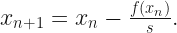
There is another straightforward way of modifying Newton’s method, which happens to be quite useful in certain circumstances. It is called the generalized Newton method, in which we take Newton’s method and instead of updating our guess to wherever the tangent line hits zero, we take that distance and scale it by some amount, $\alpha>0$ . In equation form,

$x_{n+1} = x_{n} - \alpha\frac{f(x_n)}{s}.$

Of course, when we set $\alpha = 1$ , we get back to the usual Newton’s method.

When we think of roots of a function, we often think of roots that behave linearly as they cross 0, but this is a very limited view. In general, the part of a function near a root is pretty well-approximated by a power of $(x-r)$ , where $r$ is the root’s location. Some examples are shown in the picture below.

Three graphs, each of a different function. Each graph shows a single root of the function, which has an orange box drawn around it. On the left graph it is written that the function looks linear near the root. On the middle graph, it is written that the function looks like a quadratic near the root. Finally on the right graph, it is noted that the function looks like a cubic near the root. — From left to right, the function near the root appears linear (multiplicity 1), quadratic (multiplicity 2), and cubic (multiplicity 3), respectively

We call the exponent of this approximation the multiplicity of the root. For roots with multiplicity 1, Newton’s method converges quite quickly. However, for roots with higher multiplicity, Newton’s method converges more slowly. The generalized Newton method fixes this issue. We can recover the speed at which Newton’s method normally converges by tuning $\alpha$ to the multiplicity of the root. Here is an example, where we have 3 roots of multiplicity 2, by simply taking $f(x) = (x^3 - 1)^2$ . By squaring this polynomial, we double the multiplicity of its roots. Below is the usual Newton fractal and the generalized Newton fractal for this function, colored by the number of steps it takes to converge to a root, like we did before.

Newton fractal in black and white. The background is largely gray, and the fractal parts are a bright white and appear like chains coming in from three directions towards the center of the image. — Newton fractal for $f(x) = (x^3-1)^2$

Generalized Newton fractal. The background is largely a dark gray. The fractal part is a very light gray with three-fold rotational symmetry and looks less like a chain as the other, with larger links which are more teardrop shaped. — Generalized Newton fractal $(\alpha=2)$ for the function $f(x) = (x^3-1)^2$

Generalized Newton fractal $(\alpha=2)$ for the function $f(x) = (x^3-1)^2$

The image on the right is darker overall, and the darker regions around the roots are larger than those in the left image, showing the advantage of the generalized Newton method. You might notice that the image on the right looks an awful lot like the usual Newton’s fractal for the function $x^3-1$ . This is no coincidence! We can see how the generalized Newton method near a root of multiplicity $m$ produces the same behavior as the usual Newton’s method around a root at the same position, but with multiplicity 1. It requires a tiny bit of calculus, but all we need is that the slope of the tangent line for the function $A(x-r)^m$ at a point $x_n$ is given by $mA(x_n - r)^{m-1}$ ( $A$ is just a constant). Let’s say that we are near a root of multiplicity $m$ . What this means is that the function is very well approximated to be $f(x)\approx A(x-r)^m$ , for some particular value of $A$ . When we use the generalized Newton method near this root, with $\alpha=m$ , we find

$x_{n+1} = x_{n} - m\frac{f(x_n)}{s}\approx x_n -m\frac{A(x_n-r)^m}{mA(x_n-r)^{m-1}}=x_n-(x_n-r)=r$

The above is the same behavior we would get if we started with the usual Newton’s method near a root of multiplicity 1.

We can also play around with this method to see what sorts of interesting structures pop out. For example, what happens when you make $\alpha$ larger than the multiplicity of the roots of your function? Or what if you make $\alpha$ a non-integer, like 0.5 or 1.2?

Below is a video where we take the function $f(x) = x^6-1$ and animate the generalized Newton fractal as $\alpha$ sweeps through values down to around 0.2 and back up to around 2 (the value of $\alpha$ is printed on the right hand side of the video). Then, we zoom into the fractal at $\alpha\approx2$ .

I like to think of the Newton fractal of the above function as a flower with 6 petals, each having a petal chain shoot radially out from the center of the flower. As the value of $\alpha$ gets smaller, the petals and chains become quite thin. This is because we are taking such small steps that it becomes much more difficult to get sent off towards a faraway root, so the tendency to gravitate towards the geometrically closest root is stronger. Then, as the value of $\alpha$ grows again and surpasses 1, the petals and chain links grow larger, and their once smooth-seeming edges grow thornier. The growth reminds me of frost crystallizing on a window. When I look at the negative space around the flower, it starts to appear Mandelbrot-esque at these large values of $\alpha$ .

In the interest of not only showing polynomial functions, below is a gif of the generalized Newton fractal for the function $f(x) = (tan(x) - 1)^2$ , which has roots at regular intervals, and every root has multiplicity 2. It is colored by how many steps are required to find a root, similarly to what we have seen before. We sweep through values of $\alpha$ from 0.1 to 3.9, finally zooming in on the fractal at this maximum value.

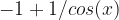
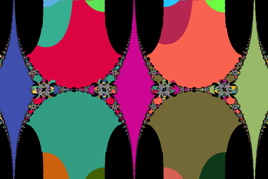
Animated gif. A horizontally-repeating gray scale fractal pattern on a white background. As the image evolves, it turns from sideways heart-shaped blobs to more flint arrowhead shapes to sideways snowman shapes, getting whiter and whiter. The fractals have long strands of smaller versions of the main fractal shooting off in different directions. The image zooms in on a snowman-shaped blob, revealing more self-similar structures dotting its boundary.

I think I will close out this post with a similar gif, this time featuring the function $-1 + 1/cos(x)$ , which has roots at every integer multiple of $\pi$ . The fractal has a similar style of coloring to before, but this one is made so that there are hardly any grays that show up.